Code
# Imports
import os
import re
import numpy as np
import pandas as pd
import xarray as xr
import matplotlib.pyplot as plt
from datetime import datetime, timedelta
from calendar import monthrange

from opendap_download import DownloadManagerTo download MERRA-2 data you need a NASA Earthdata account, your coordinates have to be converted into GEOS-5 grid indices, and the files come back as NetCDF4 blobs that need some wrangling before they’re useful.
This post walks through a Python script that handles all of that: it downloads hourly U and V wind vectors at 2m, 10m, and 50m height for one or more locations, computes wind speed from the vectors, and writes out CSV files and daily plots.
The download logic uses the merradownload package, built on Jan Urbansky’s opendap_download and Emily Laiken’s merradownload repository.
pip install merradownloadMERRA-2 data is on NASA’s GES DISC server, which requires a free Earthdata account.
The username and password from this account go into the configuration cell below.
If you want to download something other than wind, the MERRA-2 File Specification Document (PDF) lists every collection, variable name, units, and description.
# Imports
import os
import re
import numpy as np
import pandas as pd
import xarray as xr
import matplotlib.pyplot as plt
from datetime import datetime, timedelta
from calendar import monthrange
from opendap_download import DownloadManagerAll the inputs you need to change are in the next cell.
Locations are (name, latitude, longitude) tuples. Add as many as you want.
Databases. MERRA-2 splits its data across collections by type. The default here is M2T1NXSLV, the hourly single-level diagnostics collection, which has surface wind, temperature, and pressure. For radiation or solar data, swap in M2T1NXRAD / tavg1_2d_rad_Nx. The MERRA-2 File Specification Document lists everything.
Variables. U and V are the eastward and northward wind components. The suffix is the height: U10M is eastward wind at 10 metres. For temperature, T2M is 2-metre air temperature. If you change what you download here, you’ll also need to update the processing step below.
####### THE CONTROL CENTER: INPUTS - CHANGE THESE #########
username = 'YOUR-OWN-USERNAME'  # Your Earthdata Login
password = 'YOUR-OWN-PASSWORD'  # Your Earthdata Password

# WHEN do you want the data?
years = [2017]

# WHERE do you want the data? Add as many (Name, Lat, Lon) tuples as you want!
locs = [('durham', 54.7753, -1.5849)]

# WHAT DATABASE do you want to pull from?
database_name = 'tavg1_2d_slv_Nx'  # Single-level diagnostics (Wind, Temp, Pressure)
database_id = 'M2T1NXSLV'

# WHAT VARIABLES / HEIGHTS do you want from that database?
# U = Eastward wind vector, V = Northward wind vector.
# Numbers represent height (2m, 10m, 50m)
variables_to_download = ['U2M', 'V2M', 'U10M', 'V10M', 'U50M', 'V50M']

aggregator = 'mean'

####### CONSTANTS - DO NOT CHANGE BELOW THIS LINE #######
lat_coords = np.arange(0, 361, dtype=int)
lon_coords = np.arange(0, 576, dtype=int)
database_url = 'https://goldsmr4.gesdisc.eosdis.nasa.gov/opendap/MERRA2/' + database_id + '.5.12.4/'
NUMBER_OF_CONNECTIONS = 5NASA’s GEOS-5 grid uses integer indices rather than decimal degrees, so coordinates have to be mapped before querying the servers. Nothing in this section needs editing.
####### HELPER FUNCTIONS #########
def translate_lat_to_geos5_native(latitude):
    return ((latitude + 90) / 0.5)

def translate_lon_to_geos5_native(longitude):
    return ((longitude + 180) / 0.625)

def find_closest_coordinate(calc_coord, coord_array):
    index = np.abs(coord_array-calc_coord).argmin()
    return coord_array[index]

def translate_year_to_file_number(year):
    if year >= 1980 and year < 1992: return '100'
    elif year >= 1992 and year < 2001: return '200'
    elif year >= 2001 and year < 2011: return '300'
    elif year >= 2011: return '400'
    else: raise Exception('The specified year is out of range.')

def generate_url_params(parameter, time_para, lat_para, lon_para):
    parameter = list(map(lambda x: x + time_para, parameter))
    parameter = list(map(lambda x: x + lat_para, parameter))
    parameter = list(map(lambda x: x + lon_para, parameter))
    return ','.join(parameter)

def generate_download_links(download_years, base_url, dataset_name, url_params):
    urls = []
    for y in download_years:
        y_str = str(y)
        file_num = translate_year_to_file_number(y)
        for m in range(1,13):
            m_str = str(m).zfill(2)
            _, nr_of_days = monthrange(y, m)
            for d in range(1,nr_of_days+1):
                d_str = str(d).zfill(2)
                file_name = 'MERRA2_{num}.{name}.{y}{m}{d}.nc4'.format(
                    num=file_num, name=dataset_name, y=y_str, m=m_str, d=d_str)
                query = '{base}{y}/{m}/{name}.nc4?{params}'.format(
                    base=base_url, y=y_str, m=m_str, name=file_name, params=url_params)
                urls.append(query)
return urlsFor each location, this converts coordinates to GEOS-5 grid indices, builds the OPeNDAP query URLs, and downloads one file per day. A full year is 365 files, so expect a few minutes depending on your connection.
print('DOWNLOADING DATA FROM MERRA')
for loc, lat, lon in locs:
    print('Downloading data for ' + loc)
    lat_coord = translate_lat_to_geos5_native(lat)
    lon_coord = translate_lon_to_geos5_native(lon)
    lat_closest = find_closest_coordinate(lat_coord, lat_coords)
    lon_closest = find_closest_coordinate(lon_coord, lon_coords)

    requested_lat = '[{lat}:1:{lat}]'.format(lat=lat_closest)
    requested_lon = '[{lon}:1:{lon}]'.format(lon=lon_closest)

    # We use the variables_to_download list you defined in the inputs!
    parameter = generate_url_params(variables_to_download, '[0:1:23]', requested_lat, requested_lon)

    generated_URL = generate_download_links(years, database_url, database_name, parameter)

    download_manager = DownloadManager(
        username=username,
        password=password,
        download_path='WindSpeed/' + loc,
        links=generated_URL,
    )
    download_manager.start_download(NUMBER_OF_CONNECTIONS)
DOWNLOADING DATA FROM MERRA
Downloading data for durham100%|██████████| 365/365 [04:31<00:00, 1.35file/s]MERRA-2 gives you U and V wind components separately. Wind speed is their vector magnitude: \(\sqrt{U^2 + V^2}\).
If you swapped in a scalar variable like T2M for temperature, update the calculations below — pull the column directly instead of computing a magnitude.
######### OPEN, CLEAN, MERGE, AND WRITE CSVS ##########
def extract_date(data_set):
    if 'HDF5_GLOBAL.Filename' in data_set.attrs:
        f_name = data_set.attrs['HDF5_GLOBAL.Filename']
    elif 'Filename' in data_set.attrs:
        f_name = data_set.attrs['Filename']
    else:
        raise AttributeError('The attribute name has changed again!')
    exp = r'\.(\d{8})\.nc4'
    res = re.search(exp, f_name).group(1)
    y, m, d = res[0:4], res[4:6], res[6:8]
    date_str = ('%s-%s-%s' % (y, m, d))
    data_set = data_set.assign(date=date_str)
    return data_set

print('CLEANING AND MERGING DATA')
for loc, lat, lon in locs:
    print('Cleaning and merging data for ' + loc)
    dfs = []
    file_path = 'WindSpeed/' + loc

    os.makedirs(file_path, exist_ok=True)

    for file in os.listdir(file_path):
        if '.nc4' in file:
            try:
                with xr.open_mfdataset(file_path + '/' + file, preprocess=extract_date) as df:
                    dfs.append(df.to_dataframe())
            except Exception as e:
                print('Issue with file ' + file + ' | Error: ' + str(e))

    if len(dfs) == 0:
        print("No data downloaded!")
        continue

    df_hourly = pd.concat(dfs)
    df_hourly = df_hourly.reset_index()

    # --- IF YOU CHANGED VARIABLES, UPDATE THIS SECTION ---
    # Calculate actual wind speed for all three heights
    df_hourly['WindSpeed_2m'] = np.sqrt(df_hourly['U2M']**2 + df_hourly['V2M']**2)
    df_hourly['WindSpeed_10m'] = np.sqrt(df_hourly['U10M']**2 + df_hourly['V10M']**2)
    df_hourly['WindSpeed_50m'] = np.sqrt(df_hourly['U50M']**2 + df_hourly['V50M']**2)

    df_hourly['time'] = df_hourly['time'].dt.time
    df_hourly['date'] = pd.to_datetime(df_hourly['date'])

    # Extract the date, time, and all three wind speeds
    df_output = df_hourly[['date', 'time', 'WindSpeed_2m', 'WindSpeed_10m', 'WindSpeed_50m']]
    df_output.to_csv(file_path + '/' + loc + '_hourly.csv', index=False)

    # Define how to aggregate all three columns
    agg_dict = {'WindSpeed_2m': aggregator, 'WindSpeed_10m': aggregator, 'WindSpeed_50m': aggregator}
    # -----------------------------------------------------

    df_daily = df_output.groupby('date').agg(agg_dict)
    df_daily['date'] = df_daily.index
    df_daily.to_csv(file_path + '/' + loc + '_daily.csv', index=False)

    df_weekly = df_daily.copy()
    df_weekly['Week'] = pd.to_datetime(df_weekly['date']).apply(lambda x: x.isocalendar()[1])
    df_weekly['Year'] = pd.to_datetime(df_weekly['date']).apply(lambda x: x.year)
    df_weekly = df_weekly.groupby(['Year', 'Week']).agg(agg_dict).reset_index()
    df_weekly.to_csv(file_path + '/' + loc + '_weekly.csv', index=False)
CLEANING AND MERGING DATA
Cleaning and merging data for durhamReads the daily CSV and plots wind speed at all three heights. If you changed the variables above, update the column names here to match.
######### PLOT THE DATA ##########
print('PLOTTING DATA')
for loc, lat, lon in locs:
    file_path = 'WindSpeed/' + loc

    csv_file = file_path + '/' + loc + '_daily.csv'
    if not os.path.exists(csv_file):
        print(f"Skipping plot for {loc} - data file not found.")
        continue

    # Load the daily averaged data we just created
    df_plot = pd.read_csv(csv_file)
    df_plot['date'] = pd.to_datetime(df_plot['date'])

    plt.figure(figsize=(14, 6))

    # Plot the three lines
    plt.plot(df_plot['date'], df_plot['WindSpeed_50m'], label='50m Wind Speed', color='#1f77b4', linewidth=1.5, alpha=0.9)
    plt.plot(df_plot['date'], df_plot['WindSpeed_10m'], label='10m Wind Speed', color='#ff7f0e', linewidth=1.5, alpha=0.8)
    plt.plot(df_plot['date'], df_plot['WindSpeed_2m'], label='2m Wind Speed', color='#2ca02c', linewidth=1.5, alpha=0.7)

    plt.title(f'Daily Mean Wind Profile for {years[0]} - {loc.capitalize()}', fontsize=14, fontweight='bold')
    plt.xlabel('Date', fontsize=12)
    plt.ylabel('Wind Speed (m/s)', fontsize=12)
    plt.legend(loc='upper right', framealpha=1)
    plt.grid(True, linestyle='--', alpha=0.6)

    plt.tight_layout()
    plot_file = file_path + '/' + loc + '_wind_profile_plot.png'
    plt.savefig(plot_file, dpi=300)
    print(f'Saved graph to: {plot_file}')

    plt.show()

print('FINISHED')
PLOTTING DATA
Saved graph to: WindSpeed/durham/durham_wind_profile_plot.png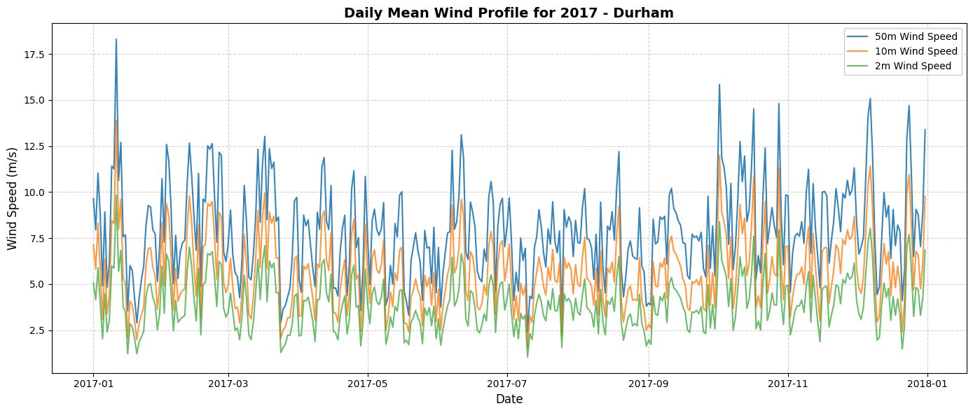
FINISHED